Simulator
To show our protocol in action, we provide a downloadable simulator. It can be configured with custom topologies and many of the key parameters of the algorithm are customizable.
Interface
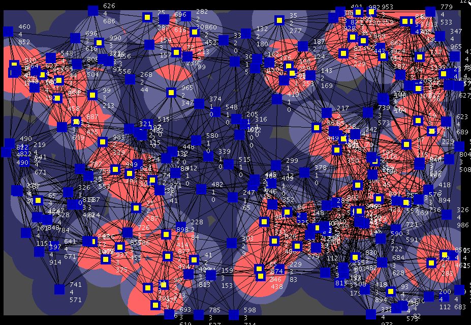
The simulator interface shows each node as a small square. The circular sensing area around each node is drawn with a circle. When the node is active (awake), its center is yellow and its sensing area highlighted. When the same area is sensed by two nodes which are active at the same time, it is colored "reddish".
Connectivity between nodes is represented by black lines.
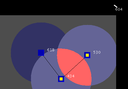
In the image above, the leftmost and rightmost nodes are not connected -- however, their sensing areas partially overlap. The current time in the epoch is shown at the upper-right corner of the interface, and cycles with a 3-second period. In the represented configuration, at time 604 the two rightmost nodes are active simultaneously, and the intersection of their sensing areas is highlighted; whereas the leftmost sensor will wake up after 14/1000 of an epoch. When placing the mouse pointer over a node, the "clock" in the upper-right corner graphically shows the part of the epoch during which the node is active.
Tutorial
Right-click to create nodes. They can be dragged around and
deleted by dropping them outside the grey rectangular area. The
wakeup time of new nodes is initialized randomly. At any time,
pressing r randomizes the
wakeup time of all sensors.
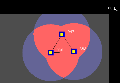
The figure depicts a rather unfortunate initialization: the three sensors wake up almost simultaneously, and leave most of the epoch uncovered. You can compute the performance measures for the current configuration by pressing m: after a while, the simulator reports data for sensing coverage, average waiting time, time to root and the average number of neighbors. Note that the first two measures are subject to a small statistical noise.
You can run a single calibration iteration by pressing s; note that
in the simulator the calibration happens instantaneously, whereas in a
real implementation it would have needed one or two epochs. After
few iterations the configuration stabilizes as follows:
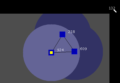
Compare the new performance measures with the previous ones: sensing coverage has improved (because areas simultaneously covered by multiple sensors are minimized). Also, average waiting time has decreased.
Clear everything with BACKSPACE
and create a sensor grid with g:
then
SHIFT-click any node in order to build
a tree from there. Now additional information is displayed near each
sensor: the level of the node in the tree (0 is the root/collection point) and
the time a message sent by the node at the end of its awake period takes to
reach the root (time to root).
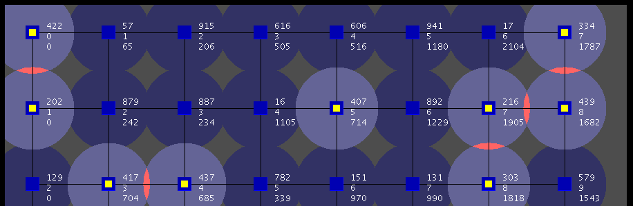
The figure shows a tree rooted on the top-left node. Note that the time to root values usually (but not always) increase with the depth in the tree. The tree is automatically destroyed as soon as any potentially topology-changing operation is performed.
The average time to root over all nodes is computed by pressing m. In presence of a tree, calibration iterations implement the probabilistic "jumping" behavior with a fixed beta=.6. Also, the gamma parameter can be tuned with q, a, z and x in order to generate a "waving" pattern towards the root, dramatically decreasing time to root while negatively affecting other performance measures.
To observe this, try setting gamma=.1 with z then triggering several calibration iterations.
The simulator handles arbitrarily complex topologies with hundreds of
nodes: have fun!
Usage
Basic operation
Run the jar with a recent JVM. Insert nodes with right mouse button, move nodes by dragging. Drag nodes outside the gray area to delete them, or use BACKSPACE to delete all nodes. r randomizes wakeup times for all nodes; s triggers a single calibration iteration; m prints performance measures of the current configuration. SHIFT + left click on a node builds a tree from there.
Other keystrokes
- n and b tune radio range
- v and c tune sensing range (for all displayed nodes)
- l and p tune awake time (for all displayed nodes)
- q and a tune gamma, z and x sets gamma to 0.1 and inf (for all displayed nodes)
- i adds a number of nodes in a connected topology
- any digit adds 50 pseudorandomly-placed nodes (with repeatable seed)
- g adds a grid of nodes
- f disables screen update (for
simulation efficiency or taking screenshots)